Decode binary region of interest

An example of gclda.decode.decode_roi.

Start with the necessary imports

from os.path import join
import matplotlib.pyplot as plt

from nilearn import plotting
from nltools.mask import create_sphere

from gclda.model import Model
from gclda.decode import decode_roi
from gclda.utils import get_resource_path

Load model and initialize decoder

model_file = join(get_resource_path(), 'models/Neurosynth2015Filtered2',
                  'model_200topics_2015Filtered2_10000iters.pklz')
model = Model.load(model_file)

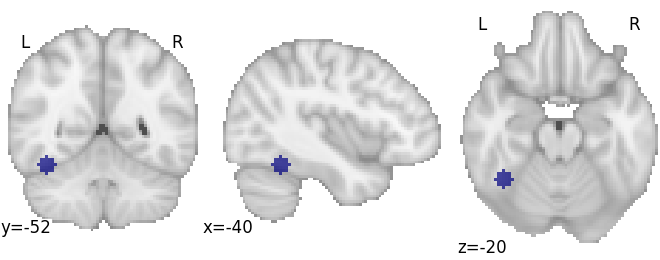
Create region of interest (ROI) image

coords = [[-40, -52, -20]]
radii = [6] * len(coords)

roi_img = create_sphere(coords, radius=radii, mask=model.dataset.mask_img)
fig = plotting.plot_roi(roi_img, display_mode='ortho',
                        cut_coords=[-40, -52, -20],
                        draw_cross=False)

Decode ROI

df, topic_weights = decode_roi(model, roi_img)

Get associated terms

df = df.sort_values(by='Weight', ascending=False)
print(df.head(10))

Out:

Weight
Term
face         14.715405
faces        11.750837
words         2.923485
visual        2.515097
word          2.102416
facial        1.315064
color         1.289241
identity      1.032067
recognition   0.973896
selectivity   0.871821

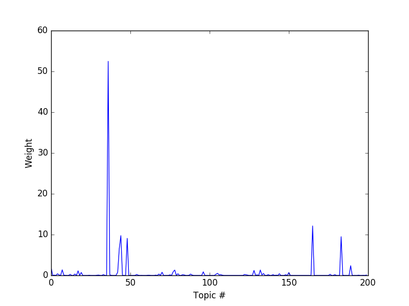
Plot topic weights

fig2, ax2 = plt.subplots()
ax2.plot(topic_weights)
ax2.set_xlabel('Topic #')
ax2.set_ylabel('Weight')
fig2.show()

Total running time of the script: ( 0 minutes 40.769 seconds)